

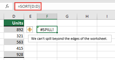
The spilled array formula you're attempting to enter extends beyond the worksheet's range. Try again with a smaller range or array.
In the following example, moving the formula to cell F1 resolves the error, and the formula spills correctly.
Common cause: Full column references
A common misunderstanding occurs when creating VLOOKUP formulas by overspecifying the lookup_value argument. Before dynamic array capable Excel, Excel only considered the value on the same row as the formula and ignored any others, as VLOOKUP expected only a single value. With the introduction of dynamic arrays, Excel considers all the values provided to the lookup_value. This change means that if you specify an entire column as the lookup_value argument, Excel attempts to look up all 1,048,576 values in the column. After it finishes, it tries to spill them to the grid, and it very likely reaches the end of the grid, resulting in a #SPILL! error.
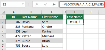
For example, when placed in cell E2 as in the following example, the formula =VLOOKUP(A:A,A:C,2,FALSE) previously looked up only the ID in cell A2. However, in dynamic array Excel, the formula causes a #SPILL! error because Excel looks up the entire column, returns 1,048,576 results, and reaches the end of the Excel grid.
Use one of the following approaches to resolve this issue:
| # | Approach | Formula |
|---|---|---|
| 1 | Reference just the lookup values you're interested in. This style of formula returns a dynamic array, but doesn't work with Excel tables.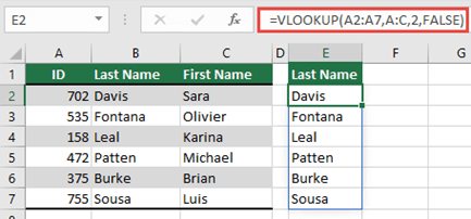
|
=VLOOKUP(A2:A7,A:C,2,FALSE) |
| 2 | Reference just the value on the same row, and then copy the formula down. This traditional formula style works in tables, but doesn't return a dynamic array.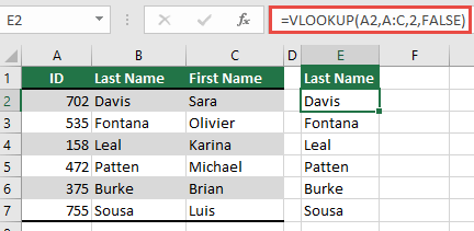
|
=VLOOKUP(A2,A:C,2,FALSE) |
| 3 | Request that Excel perform implicit intersection by using the @ operator, and then copy the formula down. This style of formula works in tables, but doesn't return a dynamic array.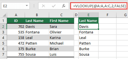
|
=VLOOKUP(@A:A,A:C,2,FALSE) |
Need more help?
You can always ask an expert in the Excel Tech Community or get support in Communities.
See Also
How to correct a #SPILL! errors