

Microsoft introduced the implicit intersection operator as part of a substantial upgrade to Excel's formula language to support dynamic arrays. Dynamic arrays bring significant new calculation ability and functionality to Excel.
Upgraded formula language
Excel's upgraded formula language is almost identical to the old language, except that it uses the @ operator to indicate where implicit intersection could occur, whereas the old language did this silently. As a result, you might notice @'s appear in some formulas when you open them in dynamic array Excel. Your formulas continue to calculate the same way they always have.
What is implicit intersection?
Implicit intersection logic reduces many values to a single value. Excel did this to force a formula to return a single value, since a cell could only contain a single value. If your formula returned a single value, implicit intersection did nothing (even though it was technically being done in the background). The logic works as follows:
- If the value is a single item, return the item.
- If the value is a range, return the value from the cell on the same row or column as the formula.
- If the value is an array, pick the top-left value.
With the advent of dynamic arrays, Excel is no longer limited to returning single values from formulas, so silent implicit intersection is no longer necessary. Where an old formula could invisibly trigger implicit intersection, dynamic array enabled Excel shows where it would have occurred with the @.
Why the @ symbol?
The @ symbol is already used in table references to indicate implicit intersection. Consider the following formula in a table =[@Column1]. The @ indicates that the formula uses implicit intersection to retrieve the value on the same row from [Column1].
Can you remove the @?
Often you can. It depends on what the part of the formula to the right of the @ returns:
- If it returns a single value (the most common case), there's no change when you remove the @.
- If it returns a range or array, removing the @ causes it to spill to the neighboring cells.
If you remove an automatically added @ and later open the workbook in an older version of Excel, it appears as a legacy array formula (wrapped with braces {}). This behavior ensures the older version doesn't trigger implicit intersection.
When do we add the @ to old formulas?
Generally, functions that return multi-cell ranges or arrays have an @ prefix if you authored them in an older version of Excel. There's no change to the way your formula behaves — you can just see the previously invisible implicit intersection now. Common functions that return multi-cell ranges include INDEX, OFFSET, and User Defined Functions (UDFs). A common exception is if they're wrapped in a function that accepts an array or range (for example, SUM() or AVERAGE()).
See Excel functions that return ranges or arrays for more details.
Examples
| Original formula | As seen in dynamic array Excel | Explanation |
|---|---|---|
| =SUM(A1:A10) | =SUM(A1:A10) | No change - No implicit intersection can occur, as the SUM function expects ranges or arrays. |
| =A1+A2 | =A1+A2 | No change - No implicit intersection can occur. |
| =A1:A10 | =@A1:A10 | Implicit intersection occurs, and Excel returns the value associated with the row the formula is in. |
| =INDEX(A1:A10,B1) | =@INDEX(A1:A10,B1) | Implicit intersection can occur. The INDEX function can return an array or range when its second or third argument is 0. |
| =OFFSET(A1:A2,1,1) | =@OFFSET(A1:A2,1,1) | Implicit intersection can occur. The OFFSET function can return a multi-cell range. When it does, it triggers implicit intersection. |
| =MYUDF() | =@MYUDF() | Implicit intersection can occur. Create custom functions in Excel can return arrays. When they do, the original formula triggers implicit intersection. |
Using the @ operator in new formulas
If you author or edit a formula in dynamic array Excel that contains the @ operator, it might appear as _xlfn.SINGLE() in pre-dynamic array Excel.
This behavior occurs when you commit a mixed formula. A mixed formula is a formula that relies on both array calculation and implicit intersection. Pre-dynamic array Excel doesn't support this combination. Pre-dynamic array Excel only supports formulas that do i) implicit intersection or ii) array calculation throughout.
When dynamic array enabled Excel detects the creation of a mixed formula, it proposes a variation of the formula that uses implicit intersection throughout. For example, if you enter =A1:A10+@A1:A10, you see the following dialog:
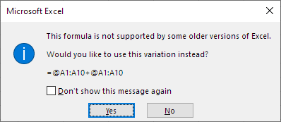
If you choose to reject the formula proposed by the dialog, the mixed formula =A1:A10+@A1:A10 is committed. If you later open this formula in pre-dynamic array Excel, it appears as =A1:A10+_xlfn.SINGLE(A1:A10) with the @ operators in the mixed formula appearing as _xlfn.SINGLE(). When pre-dynamic array Excel evaluates this formula, it returns a #NAME! error value.
Need more help?
You can always ask an expert in the Excel Tech Community or get support in Communities.